Getting Started
Contents
Getting Started#
Installation#
We recommend installing PyePAL in a dedicated virtual environment or conda environment. Note that we currently support Python 3.7 and 3.8.
To install the latest stable release use
pip install pyepal
or the conda channel (recommended)
conda install pyepal -c conda-forge
The latest version of PyePAL can be installed from GitHub using
pip install git+https://github.com/kjappelbaum/pyepal.git
On macOS you might need to install libomp (e.g., brew install libomp) for multihreading in some models.
If you want to limit how many CPUs openblas uses, you can export OPENBLAS_NUM_THREADS=1
Which class do I use?#
For Gaussian processes built with
sklearnusePALSklearnFor Gaussian processes built with
GPyusePALGPyFor coregionalized Gaussian processes (built with
GPy) usePALCoregionalizedFor quantile regression using
LightGBMgradient boosted decision trees usePALGBDTFor infinite wide neural networks with the neural tangent kernel or exact Bayesian inference (Novak et al., 2019) use
PALNTFor an ensemble of finite width neural networks (Lakshminarayanan et al., 2017) (built with JAX) use
PALNTEnsemble
If your favorite model is not listed, you can easily implement it yourself (see Implementing a new PAL class)!
Running an active learning experiment#
The examples directory contains a Jupyter notebook with an example that can also be run on MyBinder.
If using a Gaussian process model built with sklearn or GPy we recommend using a pre-built class such as PALSklearn, PALCoregionalized, PALGPy and following the subsequent steps (for more details on which class to use see Which class do I use?):
For each objective create a model (if using a coregionalized Gaussian process model, only one model needs to be created)
Sample a few initial points from the design space. We provide the
get_maxmin_samples()orget_kmeans_samples()utilities that can help with the sampling. Our code assumes thatXis anp.array.from pyepal import get_kmeans_samples, get_maxmin_samples # This selects the 10 points closest to the centroids of a k=10 means clustering indices = get_kmeans_samples(X, 10) # This selects the 10 farthest points in feature space indices = get_maxmin_samples(X, 10)
Now we can initialize the instance of one
PALclass. If using asklearnGaussian process model, we would usefrom pyepal import PALSklearn # Each of these models is an instance of sklearn.gaussian_process.GaussianProcessRegressor models = [gpr0, gpr1, gpr2] # We always need to provide the feature matrix (X), a list of models, and the number of objectives palinstance = PALSklearn(X, models, 3) # Now, we can also feed in the first measurements # this here assumes that we have all measurements for y and we now # provide those which are present in the indices array palinstance.update_train_set(indices, y[indices]) # Now we can run one step next_idx = palinstance.run_one_step()
At this level, we have a range of different optional arguements we can set.
epsilon: one \(\epsilon\) per dimension in anp.ndarray. This can be used to set different tolerances for each objective. Note that \(\epsilon_i \in [0,1]\).delta: the \(\delta\) hyperparameter (\(\delta \in [0,1]\)). Increasing this value will speed up the convergence.beta_scale: an empirical scaling parameter for \(\beta\). The theoretical guarantees in the PAL paper are derived for this parameter set to 1. But in practice, a much faster convergence can be achieved by setting it to a number \(0< \beta_\mathrm{scale} \ll 1\).goal: By default, PyePAL assumes that the goal is to maximize every objective. If this is not the case, this argument can be set using a list of “min” and “max” strings, with “min” specifying whether to minimize the ith objective and “max” indicating whether to maximize this objective.coef_var_threshold: By default, PyePAL will not consider points with a coefficient of variation \(\ge 3\) for the classification step of the algorithm. This is meant to avoid classifying design points for which the model is entirely unsure. This tends to happen when a model is severely overfit on the training data (i.e., the training data uncertainties are very low, whereas the prediction uncertainties are very high). To change this setting, reduce this value to make the check tighter or increase it to avoid this check (as in the original implementation).
In the case of missing observations, i.e., only two of three outputs are measured, report the missing observations as np.nan. The call could look like
import numpy as np

palinstance.update_train_set(np.array([1,2]), np.array([[1, 2, 3], [np.nan, 1, 2, 0]]))
for a case in which we performed measurements for samples with index 1 and 2 of our design space, but did not measure the first target for sample 2.
Hyperparameter optimization#
Usually, the hyperparameters of a machine learning model, in particular the kernel hyperparameters of a Gaussian process regression model, should be optimized as new training data is added.
However, since this is usually a computationally expensive process, it may not be desirable to perform this at every iteration of the active learning process. The iteration frequency of the hyperparameter optimization is internally set by the _should_optimize_hyperparameters function, which by default uses a schedule that optimizes the hyperparameter every 10th iteration. This behavior can be changed by override this function.
Reclassification schedule#
A problem of the e-PAL algorithm can be the case where the initial GPR predictions are wrong. This might lead to points that are actually Pareto-efficient being confidently discarded (in case the GPR predicts with low variance a performance that is dominated by some other point). Under the assumption that the GPR predictions improve over the course of the use of the algorithm, this behavior can be mitigated by “resetting” all the classification, i.e. reconsidering discarded points. In PyePAL, we automatically do this in case there is only one point left. In general, you might want to customize this behavior, which you can do, for example, by monkey patching
from pyepal.pal.schedules import linear

def my_schedule(self):
    return linear(self.iteration, 1)

PALGPyReclassify._should_reclassify = my_schedule
or by subclassing
from pyepal.pal.schedules import linear
class PALGPyReclassify(PALGPy):
    def _should_reclassify(self):
        return linear(self.iteration, 1)
In the examples above the full design space would be re-classified each iteration.
Logging#
Basic information such as the current iteration and the classification status are logged and can be viewed by printing the PAL object
print(palinstance)

# returns: pyepal at iteration 1. 10 Pareto optimal points, 1304 discarded points, 200 unclassified points.
We also provide calculation of the hypervolume enclosed by the Pareto front with the function get_hypervolume()
hv = get_hypervolume(palinstance.means[palinstance.pareto_optimal])
Properties of the PAL object#
For debugging there are some properties and attributes of the PAL class that can be used to inspect the progress of the active learning loop.
- get the points in the design space,
x: design_spacereturns the full design space matrixpareto_optimal_points: returns the points that are classified as Pareto-efficientsampled_points: returns the points that have been sampleddiscarded_points: returns the points that have been discarded
- get the points in the design space,
get the indices of Pareto efficent, sampled, discarded, and unclassified points with
pareto_optimal_indices,sampled_indices,discarded_indices, andunclassified_indicessimilarly, the number of points in the different classes can be obtained using
number_pareto_optimal_points,number_discarded_points,number_unclassified_points, andnumber_sampled_points. The total number of design points can be obtained withnumber_design_points.hyperrectangle_sizereturns the sizes of the hyperrectangles, i.e., the weights that are used in the sampling stepmeansandstdcontain the predictions of the modelsampledis a mask array. In case one objective has not been measured its cell isFalse
Exploring a space where all objectives are known#
In some cases, we may already posess all measurements, but would like to run PAL with different settings to test how the algorithm performs.
In this case, we provide the exhaust_loop() wrapper.
from pyepal import PALSklearn, exhaust_loop
models = [gpr0, gpr1, gpr2]
palinstance = PALSklearn(X, models, 3)

exhaust_loop(palinstance, y)
This will continue calling run_one_step() until there is no unclassified sample left.
Batch sampling#
By default, the run_one_step function of the PAL classes will return a np.ndarray with only one index for the point in the design space for which the next experiment should be performed. In some situations, it may be more practical to run multiple experiments as batches before running the next active learning iteration. In such cases, we provide the batch_size argument which can be set to an integer greater than one.
next_idx = palinstance.run_one_step(batch_size=10)
# next_idx will be a np.array of length 10
Note that the exhaust_loop also supports the batch_size keyword argument
palinstance = PALSklearn(X, models, 3)

# sample always 10 points and do this until there is no unclassified
# point left
exhaust_loop(palinstance, y, batch_size=10)
Adding new points to the design matrix#
In some applications, you might want to augment the design matrix after a few iterations of PyePAL. This could be useful, for example, if you start with a coarse discretization of your design space then want to refine this grid in subsequent iterations in the relevant regions of the design space.
Adding new points to the design matrix can be easily achieved using the augment_design_matrix() function that takes the new design matrix as input. By default, it will run the current model for the new, augmented, design matrix, and re-classify all points. You can turn this behavior off using the clean_classify parameter.
Alternatively, you can use the classify flag that keeps all previous classifications. This means that if there is a point that was previously Pareto-efficient in the non-augmented design space but is now dominated by a new design point, it will no longer certainly be classified as Pareto-efficient.
Note that is important that the new points are sampled from the same distribution as the previous points in the design space. Otherwise, the model will have to deal with unexpected data shift.
Plotting a learning curve#
To plot a learning curve one can use the plot_learning_curve() function. This can be useful to estimate if the number of initial points is reasonable and to see if the model is predictive.
Caveats and tricks with Gaussian processes#
One caveat to keep in mind is that \(\epsilon\)-PAL will not work if the predictive variance does not make sense, for example, when the model is overconfident and the uncertainties for the training set is significantly lower than those for the predicted set. In this case, PyePAL will untimely, and often incorrectly, label the design points. An example situation where the predictions for an overconfident model due to a training set that excludes a part of design space is shown in the figure below
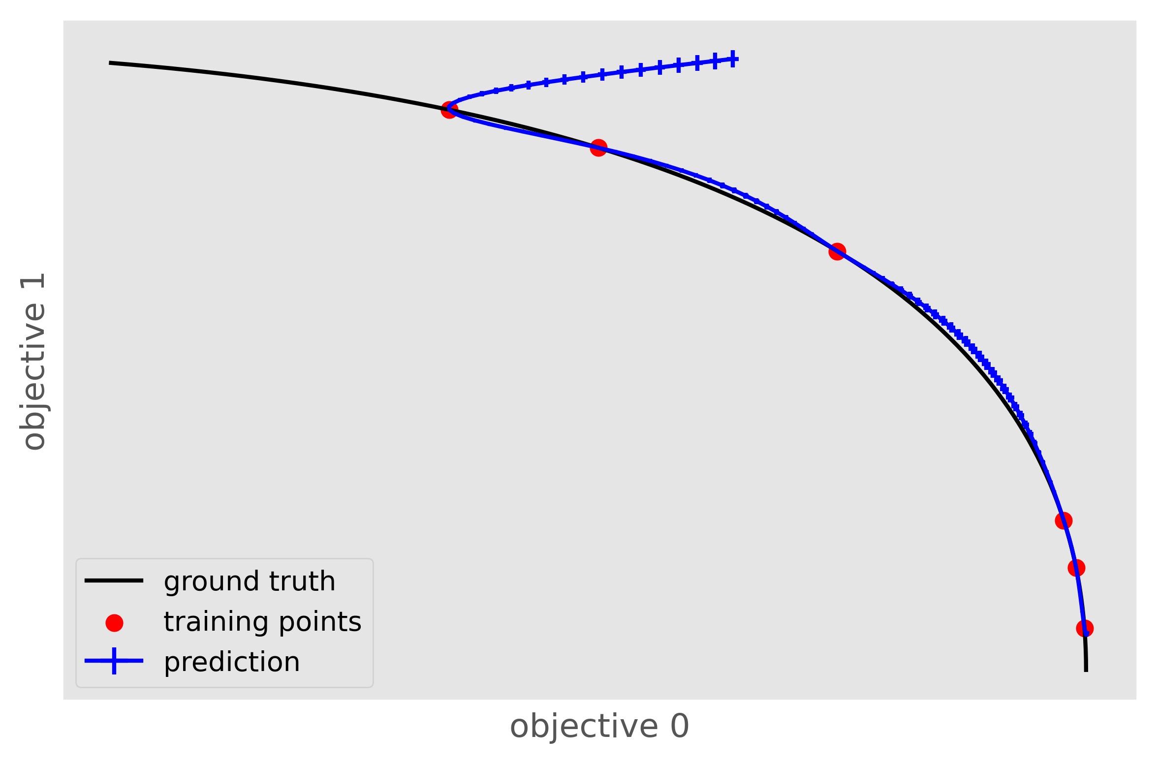
This problem is exacerbated in conjunction with \(\beta_\mathrm{scale} < 1\). To make the model more robust we suggest trying:
to set reasonable bounds on the length scale parameters
to increase the regularization parameter/noise kernel (
alphainsklearn)to increase the number of data points, especially the coverage of the design space
to turn off ARD. Automatic relevance determination (ARD) might increase the predictive performance, but also makes the model more prone to overfitting
We also recommend cross-validating the Gaussian process models and checking that the predicted variances make sense. When performing cross-validation, make sure that the index provided to PyePAL is the same size as the cross-validation folds. By default, the code will run a simple cross-validation only on the first iteration and provide a warning if the mean absolute error is above the mean standard deviation. The warning will look something like
The mean absolute error in cross-validation is 64.29, the mean variance is 0.36.
Your model might not be predictive and/or overconfident.
In the docs, you find hints on how to make GPRs more robust.
This behavior can changed with the cross-validation test being performed more frequently by overriding the should_run_crossvalidation function.
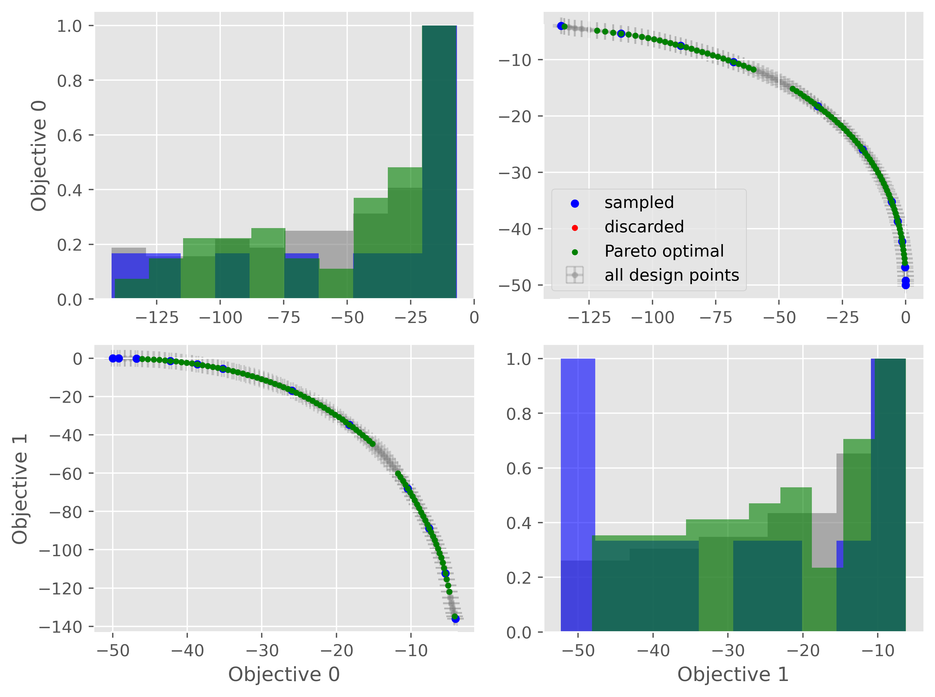
Another way to detect overfitting is to use plot_jointplot() function from the plotting subpackage. This function will plot all objectives against each other (with errorbars and different classes indicated with colors) and histograms of the objectives on the diagonal. If the majority of predicted points tend to overlap one another and get discarded by PyePAL, this may suggest that the surrogate model is overfitted.
from pyepal.plotting import plot_jointplot

# palinstance is a instance of a PAL class after
# calling run_one_step
fig = plot_jointplot(palinstance.means, palinstance)